I have been interesting in looking at my own tweets, and see what kind of visualization and analyze I could run on it. First I used the archive feature on twitter to get a file copy of my tweets, then using the package wordcloud and tm I processed the archive.

Getting a twitter snapshot

There is way to query your twitter feed directly (using API and package like twitterR) , but the simplest way I found was to download an archive. The process is quite simple, go to your Twitter account settings, there should be a Request your archive link you can click on.

It will take some time to have your snapshot ready, but when it is, you will receive an email, follow the link and download it. You can can start exploring, by opening the index.html file. The archive is quite neat, you can explore by month and have an overview of your activity over the years.

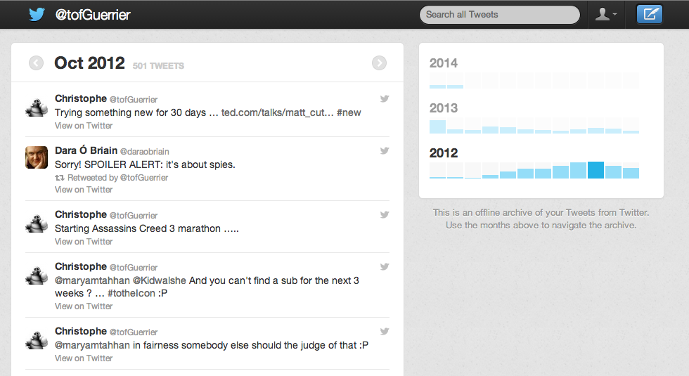
If you explore the directories unzipped the archive is composed of Json files, there is package to read those, but for my purpose I will use the csv file generated ( called tweets.csv), as I can read that straight away into R.

R processing

tweets="filepath/tweets.csv"
tw <- read.csv(file = tweets,header = TRUE)

Loading the packages I will use tm is Text Mining Package.A framework for text mining applications within R. wordcloud allow to generate word cloud pictures.

require(tm)
require(wordcloud)

From the text we create a corpus:

tw.corpus <- Corpus(DataframeSource(as.data.frame(tw$text)))

Some cleaning up of the world, I will go into more detail in part 2.

tw.corpus <- tm_map(tw.corpus, removePunctuation)
tw.corpus <- tm_map(tw.corpus, tolower)
tw.corpus <- tm_map(tw.corpus, function(x) removeWords(x, stopwords("english")))
tdm <- TermDocumentMatrix(tw.corpus)
m <- as.matrix(tdm)
v <- sort(rowSums(m),decreasing=TRUE)
d <- data.frame(word = names(v),freq=v)

Already we can find the most frequent word, i use:

max(d$freq)
d[which.max(d$freq),]$word

Which is the word via, used 458 times.

dim(d)[1]

And find that I used 14619 different words.

Plotting the word cloud is straightforward from there:

wordcloud(words = d$word,freq = d$freq,
          scale=c(8,.3),
          min.freq=10,
          max.words=dim(d)[1], random.order=T, rot.per=.15, 
          vfont=c("sans serif","plain"))

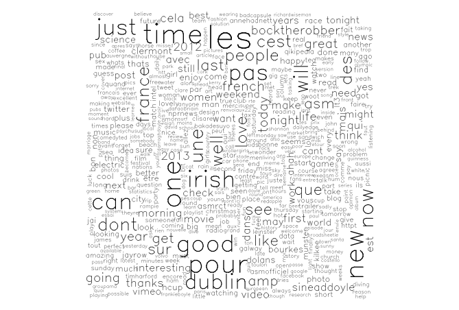
And here's the result.

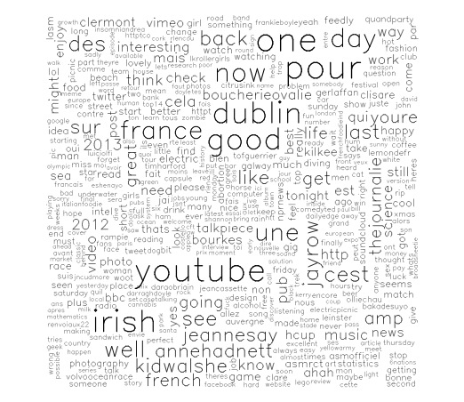
Not too bad for a first pass, but I am unhappy about few things: * the cloud could use some colours. * I can see twitter user handle in this, which is not something i want in the final cloud, it probably happen during the removing of the punctuation in the corpus processing. I will need to fix that. But that also gave the idea to create a cloud with only the user handles to visualize, who i interacted the most with. * It is very cluttered, I may need to reduce the number of words displayed, or increase the minimum limit. At the moment wordcloud tries to display every word appearing more than 10 times. * That last command, generates many warning, which need to be investigated.

We load the data and the required packages.

tw <- read.csv(file = tweets,header = TRUE)
require(tm)
require(wordcloud)

We can as previously create a corpus. In the package tm, the main data structure is an object collecting text documents. More detail can be found there: http://cran.r-project.org/web/packages/tm/vignettes/tm.pdf

I don't quite understand why, but you cannot directly input a data frame, but use a Source object - here via the appropriate command. That last command (DataframeSource) takes a data frame on convert it into the appropriate object format.

Initially I tried to put tw$text directly, but this return a list not a data frame, hence the necessary coercion.

tw.corpus <- Corpus(DataframeSource(as.data.frame(tw$text)))

Once the text are formatted in the right data structure for the package, we can avail the function of the tm package.

The most useful here for us, is tm_map, seen previously, I first remove the punctuation symbols with it, but a side effect is that all the users twitter handle lost their @ symbols. Here I want to remove the user handle all together.

My first idea was to use tm_map and removewords, meaning i had to create ( or detect ) a list of all twitter user handle.

tm_map(tw.corpus, 
  function(x) removeWords(x, grep("@[\\w\\d_]+", x=strsplit(x, split=" "), value = TRUE)))

But it seems way too complicated, and needed to deal with many exceptions around punctuation. So that not might be the best approach. At that stage I decided to change my strategy. I should the processing before creating the corpus.

Clean up time, and reload.

rm(list=ls())
tw = read.csv(file = tweets,header = TRUE)

At that stage tw$text is a list of string. I am going to merge those, remove the user handle ( actually store them in a separate list). Put all separate words into a long list

tw.txt = unlist(tw$text)
tw.words = unlist(strsplit(as.character(tw.txt), split=" "))

Extract user handles, using perl type regular expression since I am more familiar with those.

tw.usrhandle = grep("@[\\w]+", tw.words, perl = TRUE, value = TRUE) 

A bit of cleanup is necessary removing extra punctuation, again the first line would remove the @, which i want to keep, after examining the handle, there is actually only 2 symbols to remove, this is done in the second line.

#tw.usrhandle_1 = gsub("[[:punct:]]", "", tw.usrhandle)
tw.usrhandle = gsub("[\\:\\)]", "", tw.usrhandle)

We can build an barplot from that, to see the frequency of handle cited in the tweets.

barplot(table(tw.usrhandle))

For a better look, let's move to ggplot2:

require(ggplot2)
#Create a data frame for easier use
tw.usr.df = as.data.frame(table(tw.usrhandle))

ggplot(data = tw.usr.df, aes(x=tw.usrhandle, y=Freq, order=Freq)) +
  geom_bar(colour="black", fill="#DD8888", width=.7, stat="identity") +
  theme(axis.title.x = element_text(face="bold", colour="#990000", size=20),
  axis.text.x = element_text(angle=90, vjust=0.5, size=10))

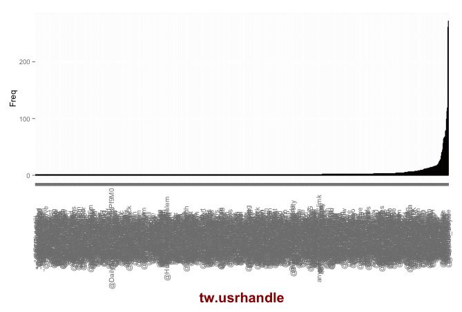
We can have a look at how many, user have been cited in the tweets, here 859.

length(unique(tw.usrhandle))

Re-ordering, by frequency, before plotting

tw.usr.df = transform(tw.usr.df, tw.usrhandle = reorder(tw.usrhandle, Freq))

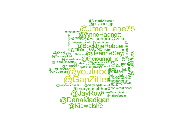
Or in a word cloud:

wordcloud(words = tw.usr.df$tw.usrhandle, 
          freq = tw.usr.df$Freq, colors=terrain.colors(20),
          min.freq = 10, max.words = Inf, random.order = TRUE)

We can do the same with hashtag, but in this case let everything down to lower case.

tw.tag = grep("#[\\w]+", tw.words, perl=TRUE, value = TRUE)
tw.tag = tolower(tw.tag)
tw.tag.df = as.data.frame(table(tw.tag))

par(bg="black")
 wordcloud(words = tw.tag.df$tw.tag, freq = tw.tag.df$Freq, colors=c("white","green","orange"),
 min.freq = 10, max.words = Inf, random.order = TRUE)
 par(bg="white")

I used 1887 tags so far, which can be found with the first line of code, we can also plot an barplot of the frequency.

length(unique(tw.tag))
ggplot(data = tw.tag.df, aes(x=tw.tag, y=Freq, order=Freq)) + 
  geom_bar(colour="black", fill="#DD8888", width=.7, stat="identity") +
  theme(axis.title.x = element_text(face="bold", colour="#990000", size=20),axis.text.x  = element_text(angle=90, vjust=0.5, size=10))

Let's go back to the words used

  tw.words.wo.usr = tw.words

Remove all usr handle

  tw.words.wo.usr[which(tw.words.wo.usr %in% tw.usrhandle)] = ""

Remove all hashtags

  tw.words.wo.usr[which(tw.words.wo.usr %in% tw.tag)] = ""

par(bg="black")
wordcloud(words = tw.words.wo.usr.df$tw.words.wo.usr, freq = tw.words.wo.usr.df$Freq, colors=c("white","green","orange"),
min.freq = 10, max.words = Inf, random.order = TRUE)
par(bg="white")

But this generate a word cloud where we can see loads of english stopword like "the", "a" ... etc

This is where tm makes life easier. So time to go back to a corpus and the tm package. Now we have a vector as input, so we use a different construct

tw.corpus = Corpus(VectorSource(tw.words.wo.usr))

Here is can basically reuse the same code from last, I wrap it around a function, to make it easier to use in the future - should have started with that to be fair.

process_corpus = function(tw.corpus){
 tw.corpus = tm_map(tw.corpus, removePunctuation)
 tw.corpus = tm_map(tw.corpus, tolower)
 tw.corpus = tm_map(tw.corpus, function(x) removeWords(x, stopwords("english")))
 tdm = TermDocumentMatrix(tw.corpus)
 m = as.matrix(tdm)

And run the function

d = process_corpus(tw.corpus)

Finally plotting the wordcloud

wordcloud(words = d$word,freq = d$freq,
 scale=c(8,.3),
 min.freq=10,
 max.words=Inf, random.order=T, rot.per=.15, 
 vfont=c("sans serif","plain"))

In summary, few lessons:

it's worth to spend some time to process the data, to put it in a form usable. It can be a tedious process, but once you have the data in the right format, the function and package available in R makes your life really easy.

Write functions as much as you can, and as early as possible, instead of writing or copying te same lines of code over and over.

So I have produced nice graphs ( well I think so), but i haven't told any story, so it's a bit pointless.

A couple of links which were very useful in writing the R code:

Mining twitter with R.

Text mining with tm.